Discriminative Classification
Decision Trees and Random Forests
This page can be downloaded as interactive jupyter notebook
In this notebook, we implement two discriminative classification models - Decision Tree and Random Forest - using Python and the scikit-learn library. We start with the decision trees, since a random forest is basically a combination of multiple decision trees and thus builds up on those.
A decision tree can be seen as a graph structure, where each node corresponds to one decision except for the leave nodes that correspond to a class (or a class distribution). We illustrate this with the following example. Assume we have set of red and blue marbles and we want to build a machine that sorts those marbles according to their colors. The machine has one marble input and two outputs (one for each class / colour). We further introduce a decision node that checks the color of each marble and forwards it to the left or the right, depending on the outcome of the check. Our sorting machine is illustrated in the next figure:

For simplicity, we change to a lighter way of illustrating the decision trees. Depicted as a graph our decision tree would look like this:
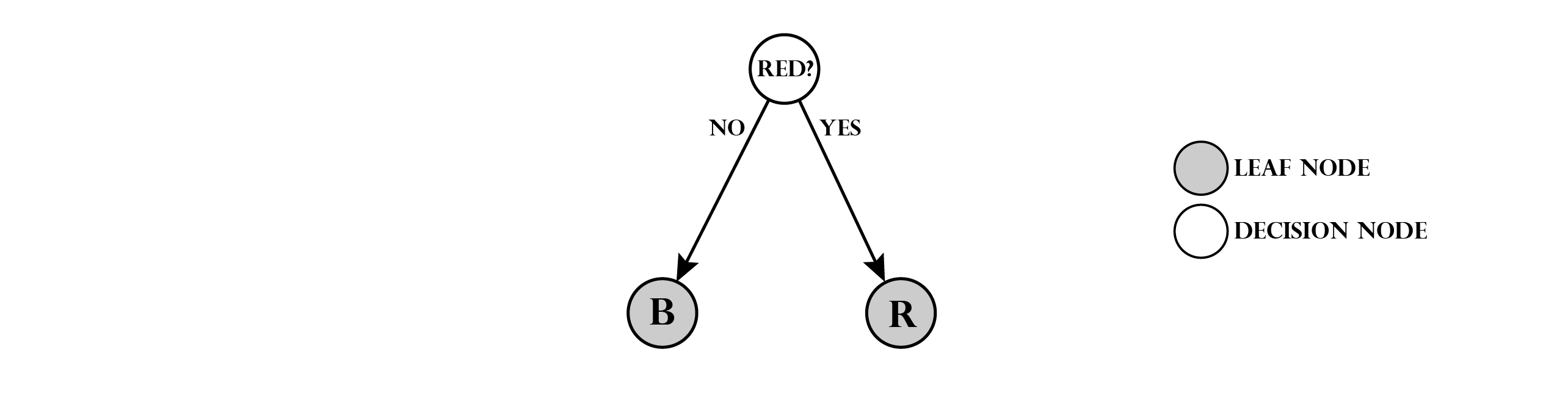
Note that we have two types of nodes: decision nodes and leaf nodes (shaded). Leaf nodes indicate, that we assign the stored class to any marble that reaches this position. To make the task a little more complex, we add a third class: green marbles (G). In order to predict this class, we modify the tree:
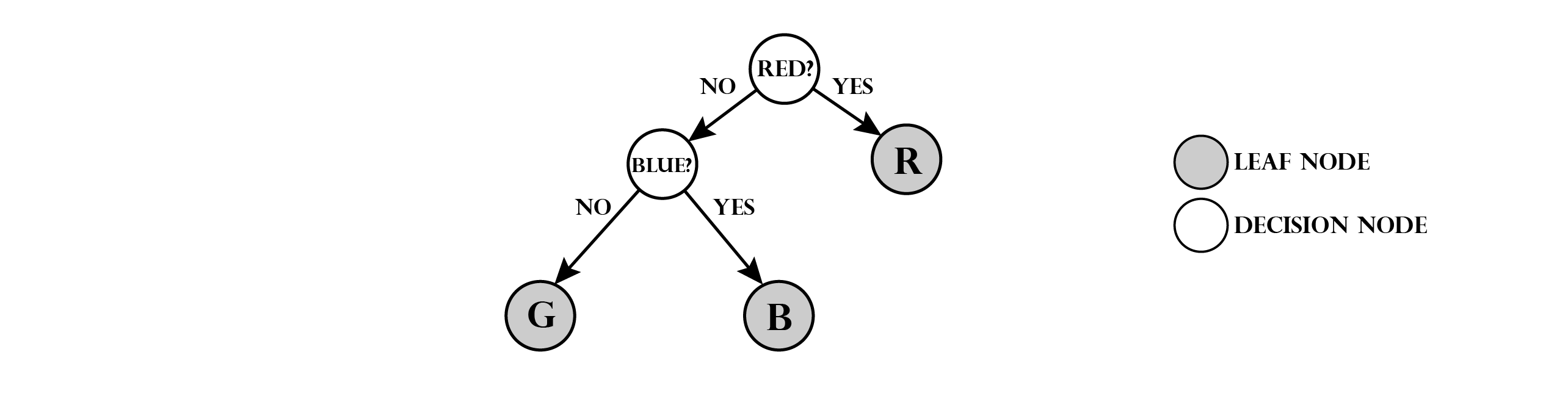
The tree has now a maximum depth of two, since two checks are required to identify a green or blue marble. Note that the ordering and type of checks is not unique. E.g. first checking if a marble is green and if not checking for red would also be valid.
In general a decision tree contains of an arbitrary number of decisions, classifying objects with arbitrary attributes. In the above example we only checked for a certain colour, but in general any operation with a boolean outcome (True or False) could be used as a decision node.
The training procedure will not be covered in detail here, but in general a set of training data is used to determine well separating decision criteria. Usually for each node multiple random criteria are used and the one which results in the highest information gain is kept.
Preparation
In order to implement the methods, we import the required Python modules:
import numpy as np                                   # Used for numerical computations
import matplotlib.pyplot as plt                      # Plotting library
from sklearn.ensemble import RandomForestClassifier

# This is to set the size of the plots in the notebook
plt.rcParams['figure.figsize'] = [6, 6]
Creating a Toy Dataset
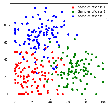
Next, we will create a toy dataset. It will contain samples which are drawn from 3 normal distributions, where each distribution represents a class.
num_c = 3 # Number of clusters
colours = [[255, 170, 170], [170, 255, 170], [170, 170, 255]]

# Generate the samples (3 clusters), we set a fixed seed make the results reproducable
np.random.seed(0)
c1_samples = np.clip([(20, 20) + np.random.randn(2)*15 for i in range(100)], 0, 100)
c2_samples = np.clip([(70, 30) + np.random.randn(2)*15 for i in range(100)], 0, 100)
c3_samples = np.clip([(30, 70) + np.random.randn(2)*15 for i in range(100)], 0, 100)

# Plot the samples, colored by class
plt.scatter(*zip(*c1_samples), c='red', marker='o', label='Samples of class 1')
plt.scatter(*zip(*c2_samples), c='green', marker='o', label='Samples of class 2')
plt.scatter(*zip(*c3_samples), c='blue', marker='o', label='Samples of class 3')
plt.legend()
plt.show()
We stack all data samples to one matrix and append the class index as additional column. Each row in the resulting matrix contains one the x and y coordinates and the class index of one sample.
c1_array = np.hstack((np.array(c1_samples), 1 * np.ones((len(c1_samples), 1))))
c2_array = np.hstack((np.array(c2_samples), 2 * np.ones((len(c2_samples), 1))))
c3_array = np.hstack((np.array(c3_samples), 3 * np.ones((len(c3_samples), 1))))

all_samples = np.vstack((c1_array, c2_array, c3_array))
print('Shape of stacked sample matrix:', all_samples.shape)
Shape of stacked sample matrix: (300, 3)
Decision Tree
Now that we have a data set we continue with the implementation of a decision tree in Python. We implement everything from scratch only using numpy for working with numerical arrays. We start with modelling decision criterions. For simplicity, in each decision either the x or y coordinate is compared to a threshold e.g. x > 50 or y < 25. We therefore can model any criterion with a tuple of three attributes:
greater: boolean variable that indicates our operator (if true the operator is>if False it’s<)threashold: the threshold value to compare withfeature: denotes the feature index (in this case either 0 forxor 1 fory)
Using this model, we can implement the following two functions. The first one will create a random criterion (used during training), the second one evaluates a criterion and returns the boolean result. Note that for simplicity the range of the random threshold is already adjusted to the toy data set.
def get_random_criterion():
    greater = np.random.random() > 0.5
    threshold = np.random.random() * 100   # here we use knowledge about the data set!
    feature = np.random.randint(0, 2)      # here we use knowledge about the feature dimensionality!
    return [greater, threshold, feature]

def eval_criterion(criterion, vector):
    g, t, f = criterion
    return (vector[f] < t) ^ g
We further need two helper functions that compute the entropy of a data set and the information gain of a criterion with respect to a set of features. Information gain is defined as
$\Delta E = \dfrac{N_1}{N_1+N_2}\cdot \sum\limits_k P_1(L^k)\cdot log_2 [P_1(L^k)] + \dfrac{N_2}{N_1+N_2}\cdot \sum\limits_k P_2(L^k)\cdot log_2 [P_2(L^k)] $
where the index denotes the subsets 1 and 2 that result from a criterion. The sums correspond to the entropy of the subsets histogram.
def get_entropy(data):
    class_counts = np.bincount(data[:,2].astype(np.int))
    P = class_counts / np.sum(class_counts)
    P = P[P > 0]
    return np.sum(P * np.log2(P))

def get_inf_gain(criterion, data):
    outcomes = np.array([eval_criterion(criterion, vector) for vector in data])
    set1 = data[outcomes]
    set2 = data[np.logical_not(outcomes)]
    N1, N2 = len(set1), len(set2)
    return N1/(N1+N2)*get_entropy(set1) + N2/(N1+N2)*get_entropy(set2)
Next, we implement the nodes.
class Node():
    n_id = 1
    def __init__(self, leaf):
        self.is_leaf = leaf
        self.criterion = None
        self.successor_yes = None
        self.successor_no = None
        self.label = None
        self.id = Node.n_id
        Node.n_id += 1
        self.is_trained = False
        self.train_samples = []

    def set_successor(self, node, yes_branch):
        if yes_branch: self.successor_yes = node
        else: self.successor_no = node

    def predict(self, vector):
        if eval_criterion(self.criterion, vector):
            return self.successor_yes
        else:
            return self.successor_no

    def train(self):
        if self.is_leaf or all(self.train_samples[:,2]==self.train_samples[0,2]):
            self.is_leaf=True
            self.label = np.argmax(np.bincount(self.train_samples[:,2].astype(np.int)))
            self.truncate()
        else:
            criteria = [get_random_criterion() for i in range(1000)]
            scores = np.array([get_inf_gain(criterion, self.train_samples) for criterion in criteria])
            self.criterion = criteria[np.argmax(scores)]
        self.is_trained = True

    def truncate(self):

        if self.successor_yes:
            self.successor_yes.truncate()
        if self.successor_no:
            self.successor_no.truncate()
        self.is_trained=True

    def __repr__(self):
        if self.is_leaf:
            return('N{} (Leaf-Node)'.format(self.id))
        else:
            return('N{} (yes -> N{} / no -> N{})'.format(self.id,self.successor_yes.id,self.successor_no.id))
Finally we combine everything in the class DecisionTree.
class DecisionTree():
    def __init__(self, depth=3):
        self.root_node = Node(leaf = False)
        self.all_nodes = [self.root_node]
        self.layers = [[self.root_node]]
        for nl in range(1, depth):
            layer = []
            num_nodes = 2**nl
            last_layer = (nl ==(depth-1))
            for n in range(num_nodes):
                node = Node(last_layer)
                self.layers[nl-1][n//2].set_successor(node, not n%2)
                layer.append(node)
                self.all_nodes.append(node)
            self.layers.append(layer)

    def predict(self, vector):
        node = self.root_node
        while not node.is_leaf:
            node = node.predict(vector)
        return int(node.label)

    def train(self, data, verbose=False):
        while not all([node.is_trained for node in self.all_nodes]):
            # Forward training samples
            for node in self.all_nodes:
                node.train_samples = []
            for vector in data:
                node = self.root_node
                while True:
                    if node.is_trained:
                        if node.is_leaf: break
                        node = node.predict(vector)
                    else:
                        node.train_samples.append(vector)
                        break
            # Train all nodes that are not trained and have samples
            for node in self.all_nodes:
                if (not node.is_trained) and len(node.train_samples):
                    node.train_samples = np.array(node.train_samples)
                    if verbose: print('training node', node)
                    node.train()
DT = DecisionTree()
for i, layer in enumerate(DT.layers):
    print('Layer {}: {}'.format(i, layer))
Layer 0: [N1 (yes -> N2 / no -> N3)]
Layer 1: [N2 (yes -> N4 / no -> N5), N3 (yes -> N6 / no -> N7)]
Layer 2: [N4 (Leaf-Node), N5 (Leaf-Node), N6 (Leaf-Node), N7 (Leaf-Node)]
DT.train(all_samples, verbose=True)
print('training done')
training node N1 (yes -> N2 / no -> N3)
training node N2 (yes -> N4 / no -> N5)
training node N3 (yes -> N6 / no -> N7)
training node N4 (Leaf-Node)
training node N5 (Leaf-Node)
training node N6 (Leaf-Node)
training node N7 (Leaf-Node)
training done
Evaluation
To visualize the decision boundaries we predict every feature of the feature space.
def predict_feature_space_dt(model):
    label_map = np.zeros((100, 100, 3), dtype=np.ubyte)
    for x in range(100):
        for y in range(100):
            label = model.predict(np.array((x, y), dtype=np.float))
            label_map[y, x] = colours[label-1]
    return label_map
label_map_dt = predict_feature_space_dt(DT)

plt.imshow(label_map_dt)
plt.scatter(*zip(*c1_samples), c='red', marker='o', label='Samples of class 1')
plt.scatter(*zip(*c2_samples), c='green', marker='o', label='Samples of class 2')
plt.scatter(*zip(*c3_samples), c='blue', marker='o', label='Samples of class 3')
plt.title('DT (3 layer)'); plt.legend(); plt.show()
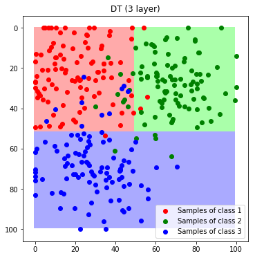
To understand the influence of the depth, we train a second tree with a depth of 7.
DT7 = DecisionTree(depth=7)
DT7.train(all_samples)
And plot the decision boundaries.
label_map_dt7 = predict_feature_space_dt(DT7)

plt.imshow(label_map_dt7)
plt.scatter(*zip(*c1_samples), c='red', marker='o', label='Samples of class 1')
plt.scatter(*zip(*c2_samples), c='green', marker='o', label='Samples of class 2')
plt.scatter(*zip(*c3_samples), c='blue', marker='o', label='Samples of class 3')
plt.title('DT (7 layer)'); plt.legend(); plt.show()
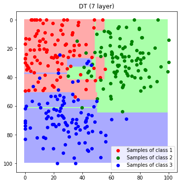
We can observe, that by increasing the number of layers the tree starts to add thin areas that correspond to outliers in the training data. This means that the model is overfitting to the training data. The choice of depth is maybe the most important parameter of a decision tree.
Random Forest
Since decision trees are prone to overfitting, as seen in the previous example, the idea of a random forest is to train multiple trees and use them jointly as an ensemble of classifiers in order to create a more robust classification model. To train a random forest, we usually train each tree with a different subset of the available training data resulting in multiple, different trees. A common way to classify a new data sample is to predict its class with each tree separately and then assign the class with the most votes.
This time we will use the scikit-learn implementation.
# set number of trees
nt = 250
cr = 'entropy'
depth = 7

# Generate the RF classifier
rf = RandomForestClassifier(n_estimators=nt, criterion=cr, max_depth=depth, bootstrap = True, n_jobs = -1)

# Train the classifier
rf.fit(all_samples[:,:2], all_samples[:,2])
RandomForestClassifier(bootstrap=True, class_weight=None, criterion='entropy',
            max_depth=7, max_features='auto', max_leaf_nodes=None,
            min_impurity_decrease=0.0, min_impurity_split=None,
            min_samples_leaf=1, min_samples_split=2,
            min_weight_fraction_leaf=0.0, n_estimators=250, n_jobs=-1,
            oob_score=False, random_state=None, verbose=0,
            warm_start=False)
Evaluation
Again, we classify each feature in the feature space to visualize the decision boundaries..
def predict_feature_space_rf(model):
    label_map = np.zeros((100, 100, 3), dtype=np.ubyte)
    feature_space = []
    for x in range(100):
        for y in range(100):
            feature_space.append((x,y))
    feature_space = np.array(feature_space)
    labels = model.predict(feature_space)
    for x in range(100):
        for y in range(100):
            label = labels[x*100+y]
            label_map[y, x] = colours[int(label)-1]
    return label_map
label_map_rf = predict_feature_space_rf(rf)

plt.imshow(label_map_rf)
plt.scatter(*zip(*c1_samples), c='red', marker='o', label='Samples of class 1')
plt.scatter(*zip(*c2_samples), c='green', marker='o', label='Samples of class 2')
plt.scatter(*zip(*c3_samples), c='blue', marker='o', label='Samples of class 3')
plt.title('RF (250 trees)'); plt.legend(); plt.show()
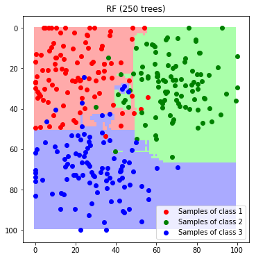
We see that, although the maximum depth is set very high, we do not observe strong overfitting.
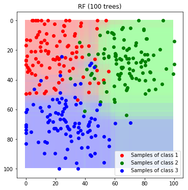
A further benefit of random forests is, that it is possible to derive probabilities from the voting statistics. In the next example we visualize the predicted probabilities instead of the final class label for the complete feature space
def predict_feature_space_rf_prob(model):
    label_map = np.zeros((100, 100, 3), dtype=np.ubyte)
    feature_space = []
    for x in range(100):
        for y in range(100):
            feature_space.append((x,y))
    feature_space = np.array(feature_space)
    probas = model.predict_proba(feature_space)
    for x in range(100):
        for y in range(100):
            proba = probas[x*100+y]
            label_map[y, x] = np.sum(colours*proba, axis=1).astype(np.ubyte)
    return label_map
label_map_rf = predict_feature_space_rf_prob(rf)

plt.imshow(label_map_rf)
plt.scatter(*zip(*c1_samples), c='red', marker='o', label='Samples of class 1')
plt.scatter(*zip(*c2_samples), c='green', marker='o', label='Samples of class 2')
plt.scatter(*zip(*c3_samples), c='blue', marker='o', label='Samples of class 3')
plt.title('RF (100 trees)'); plt.legend(); plt.show()
Discussion
Decision trees and random forests are both frequently used models. This is due to the fact that both training and evaluation is rather fast and tuning such a model is quite easy. We saw, that training a random forest requires only a few lines of code, when using the scikit-learn implementation.
| Author: | Dennis Wittich |
| Last modified: | 09.05.2019 |