RGB & HSV, color space transformations in Python
This page can be downloaded as interactive jupyter notebook
This tutorial addresses the conversion between the color spaces RGB and HSV. In comparision to the RGB color space, where each color is defined by its intensity of red, green and blue in a euclidean space, the HSV color space relies on a cylindrical coordinate system. The color attributes are saturation (how much, does the color differ from gray), intensity (how bright is the color) and hue (the angle of the color on a pre defined color wheel).
Details on the definitions can be found here.
Definitions
- R: Intensity of ‘Red’.
- G: Intensity of ‘Green’.
- B: Intensity of ‘Blue’.
- H: Color attribute ‘Hue’.
- S: Color attribute ‘Saturation’.
- V: Color attribute ‘Value’.
import numpy as np
import imageio
import matplotlib.pyplot as plt

plt.rcParams["figure.figsize"] = [18, 5]
Conversion from RGB to HSV
The following function takes an RGB image as argument (as 3D array, where the third dimension represents the three color channels) and returns the transformed image in HSV space (again a 3D array, third dimension holding the color features).
def RGB2HSV(RGB):
    RGB_normalized = RGB / 255.0                           # Normalize values to 0.0 - 1.0 (float64)
    R = RGB_normalized[:, :, 0]                            # Split channels
    G = RGB_normalized[:, :, 1]
    B = RGB_normalized[:, :, 2]

    v_max = np.max(RGB_normalized, axis=2)                 # Compute max, min & chroma
    v_min = np.min(RGB_normalized, axis=2)
    C = v_max - v_min

    hue_defined = C > 0                                    # Check if hue can be computed

    r_is_max = np.logical_and(R == v_max, hue_defined)     # Computation of hue depends on max
    g_is_max = np.logical_and(G == v_max, hue_defined)
    b_is_max = np.logical_and(B == v_max, hue_defined)

    H = np.zeros_like(v_max)                               # Compute hue
    H_r = ((G[r_is_max] - B[r_is_max]) / C[r_is_max]) % 6
    H_g = ((B[g_is_max] - R[g_is_max]) / C[g_is_max]) + 2
    H_b = ((R[b_is_max] - G[b_is_max]) / C[b_is_max]) + 4

    H[r_is_max] = H_r
    H[g_is_max] = H_g
    H[b_is_max] = H_b
    H *= 60

    V = v_max                                              # Compute value

    sat_defined = V > 0

    S = np.zeros_like(v_max)                               # Compute saturation
    S[sat_defined] = C[sat_defined] / V[sat_defined]

    return np.dstack((H, S, V))
Conversion from HSV to RGB
def HSV2RGB(HSV):
    H = HSV[:, :, 0]                                           # Split attributes
    S = HSV[:, :, 1]
    V = HSV[:, :, 2]

    C = V * S                                                  # Compute chroma

    H_ = H / 60.0                                              # Normalize hue
    X  = C * (1 - np.abs(H_ % 2 - 1))                          # Compute value of 2nd largest color

    H_0_1 = np.logical_and(0 <= H_, H_<= 1)                    # Store color orderings
    H_1_2 = np.logical_and(1 <  H_, H_<= 2)
    H_2_3 = np.logical_and(2 <  H_, H_<= 3)
    H_3_4 = np.logical_and(3 <  H_, H_<= 4)
    H_4_5 = np.logical_and(4 <  H_, H_<= 5)
    H_5_6 = np.logical_and(5 <  H_, H_<= 6)

    R1G1B1 = np.zeros_like(HSV)                                # Compute relative color values
    Z = np.zeros_like(H)

    R1G1B1[H_0_1] = np.dstack((C[H_0_1], X[H_0_1], Z[H_0_1]))
    R1G1B1[H_1_2] = np.dstack((X[H_1_2], C[H_1_2], Z[H_1_2]))
    R1G1B1[H_2_3] = np.dstack((Z[H_2_3], C[H_2_3], X[H_2_3]))
    R1G1B1[H_3_4] = np.dstack((Z[H_3_4], X[H_3_4], C[H_3_4]))
    R1G1B1[H_4_5] = np.dstack((X[H_4_5], Z[H_4_5], C[H_4_5]))
    R1G1B1[H_5_6] = np.dstack((C[H_5_6], Z[H_5_6], X[H_5_6]))

    m = V - C
    RGB = R1G1B1 + np.dstack((m, m, m))                        # Adding the value correction

    return RGB
Testing both directions
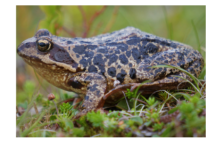
First we load an example image.
RGB = imageio.imread('./images/frog.jpg')   # Load image

plt.imshow(RGB)                             # Plot image
plt.axis('off')
plt.show()
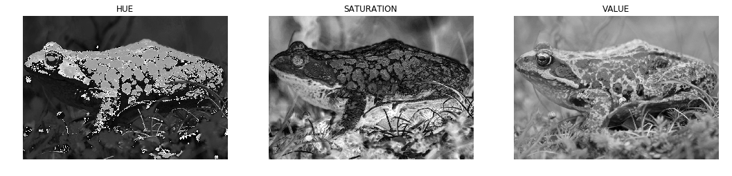
Next, we transform the image to HSV color space and display the features as gray scale images.
HSV = RGB2HSV(RGB)              # Convert RGB to HSV

HUE = HSV[:, :, 0]              # Split attributes
SAT = HSV[:, :, 1]
VAL = HSV[:, :, 2]

plt.subplot(1,3,1)              # Plot color attributes
plt.imshow(HUE, cmap='gray')
plt.title('HUE')
plt.axis('off')
plt.subplot(1,3,2)
plt.imshow(SAT, cmap='gray')
plt.title('SATURATION')
plt.axis('off')
plt.subplot(1,3,3)
plt.imshow(VAL, cmap='gray')
plt.title('VALUE')
plt.axis('off')
plt.show()
To test the transformation from HSV to RGB we apply the corresponding function and plot the result.
RGB = HSV2RGB(HSV)                                # Convert HSV back to RGB

RGB = (RGB * 255).astype(np.uint8)                # Cast back to 'byte'

plt.imshow(RGB)                                   # Plot image
plt.axis('off')
plt.show()

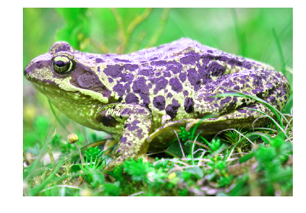
Modifications in HSV color space
In the following cell we apply some changes to the HSV features. We shift the hue value and increase the saturation and color value of each pixel. Especially a hue shift would be hard to perform on a RGB image.
HUE2 = (HUE + 45) % 360                           # Hue shift
SAT2 =  np.minimum(SAT * 1.1, np.ones_like(SAT))  # Increase saturation
VAL2 =  np.minimum(VAL * 1.4, np.ones_like(VAL))  # Increase value (brightness)

HSV2 = np.dstack((HUE2, SAT2, VAL2))              # Stack to a new HSV array
RGB2 = HSV2RGB(HSV2)                              # Convert it to RGB

RGB2 = (RGB2 * 255).astype(np.uint8)              # Cast back to 'byte'

plt.imshow(RGB2)                                  # Plot image
plt.axis('off')
plt.show()
| Author: | Dennis Wittich |
| Last modified: | 02.05.2019 |