Image representations and processing in Python
This page can be downloaded as interactive jupyter notebook
This tutorial addresses the representations of images in Python. It also covers essential image processing operations like loading and saving images.
Representations
Digital images are usually multidimensional tensors/arrays holding the intensity values of one or more channels. The first two dimensions specify the location of each pixel. According to the definition and representation of two dimensional arrays (matrices) the first dimension specifies the row and the second dimension the column of a pixel. The origin is located at the upper left corner of the image. If there is a third dimension depends on the information of the image. A gray-scale image has only one channel and thus can be represented as a 2D array. A multi-channel image holds multiple channels e.g. red, green and blue. Therefore a 3D array is required to represent such an image, where usually the third dimension represents the different channels. Of course the ordering of the axis can be changed, but most common frameworks use the row/column/channel ordering.
Additionally the order of the channels can vary as well. Where frameworks like tensorflow, matplotlib and imageio use the red/green/blue order, other frameworks like OpenCV uses the blue/green/red order by default.
Another property of the representation is the data type and value range. It is most common to use 8 bit (one byte) to encode each intensity value. This leads to a range from 0 (minimum intensity) to 255 (maximum intensity) without decimal values. When processing images and producing intermediate result, this range is often insufficient. One possibility to get a higher range is to cast the data type e.g. to 64 bit floating point numbers, which has to be undone bevor saving the image.
Definition (imageio)
According to the documentation of imageio, an image can have the following structures:
| Informations | Nr. of channels | Nr. of dimensions | Shape | Data Type | Value range |
|---|---|---|---|---|---|
| Gray values | 1 | 2 | h x w | uint8 | 0 - 255 |
| RGB (Color) | 3 | 3 | h x w x 3 | uint8 | 0 - 255 |
| RGB (Color + Alpha) | 4 | 3 | h x w x 4 | uint8 | 0 - 255 |
Here h is the height and w is the width of the image. The definition of the axis and dimensions are illustrated in the following graphic:

Loading an image from disk
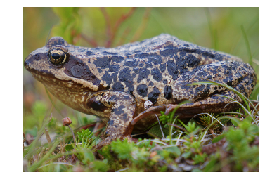
In the following example the imageio module is used to load an image from disk. Matplotlib is then used to display the image.
import imageio
import matplotlib.pyplot as plt
plt.rcParams["figure.figsize"] = [6, 30]

I = imageio.imread('images/frog.jpg')

plt.imshow(I)
plt.axis('off')
plt.show()
The imageio module uses the Numpy framework to represent the image. Knowing this, we can check some attributes of the array I which holds the image as well as some class information:
print('Class:             ', type(I))
print('Base class:        ', imageio.core.util.Image.__bases__[0])
print('-------------------')
print('Data type:         ', I.dtype)
print('Nr. of dimensions: ', I.ndim)
print('Shape:             ', I.shape)
Class:              <class 'imageio.core.util.Image'>
Base class:         <class 'numpy.ndarray'>
-------------------
Data type:          uint8
Nr. of dimensions:  3
Shape:              (700, 1000, 3)
So I is a 8 bit (0-255) per pixel array that is 700 pixel high, 1000 pixel wide and has 3 channels.
Processing examples
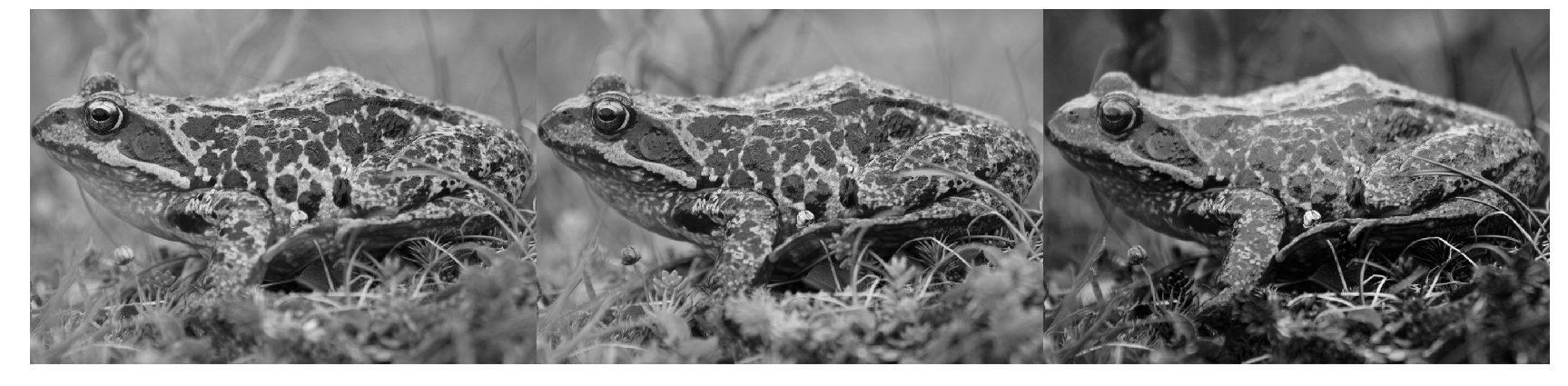
Since the image is a Numpy array, we can use all Numpy features. Exemplary we will separate and display the channels:
import numpy as np
plt.rcParams["figure.figsize"] = [30, 30]

R = I[:,:,0]
G = I[:,:,1]
B = I[:,:,2]

R_G_B = np.hstack((R,G,B))
plt.imshow(R_G_B, cmap='gray')
plt.axis('off')
plt.show()
Another common task is to create a gray-scale image from the color image, which means to compute the mean intensity for each pixel. Using np.mean will implicitly cast the data type to float64, so we will cast the result back to uint8
plt.rcParams["figure.figsize"] = [6, 30]

GV = np.mean(I, axis=2)
print('dtype after computing the mean:', GV.dtype)
GV = GV.astype(np.uint8)
plt.imshow(GV, cmap='gray')
plt.axis('off')
plt.show()
dtype after computing the mean: float64
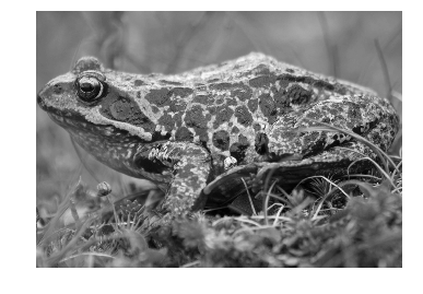
Since np.mean drops one dimension, we produced a 2D array, which is still valid in terms of imageios image definitions. We can save the image as gray-scale image:
imageio.imsave('images/frog_gray.jpg', GV)
To verify this, we will read and show the saved image again:
I_gray = imageio.imread('images/frog_gray.jpg')

print('Data type:         ', I_gray.dtype)
print('Nr. of dimensions: ', I_gray.ndim)
print('Shape:             ', I_gray.shape)

plt.imshow(I_gray, cmap='gray')
plt.axis('off')
plt.show()
Data type:          uint8
Nr. of dimensions:  2
Shape:              (700, 1000)

| Author: | Dennis Wittich |
| Last modified: | 02.05.2019 |